Denoising Diffusion Probabilistic Models

Diffusion models are latent variable models of the form $p_{\theta }:=\int p_{\theta }(x_{0:T})d{x}_{1:T}$, where $x_1,\cdots ,x_T$ are latents of the same dimensionality as the data $x_0\sim q(x_0)$. $x_0$ represents true data observations such as natural images, $x_T$ represents pure Gaussian noise, and $x_t$ is an intermediate noisy version of $x_0$. The joint distribution $p_{\theta }(x_{0:T})$ is called the reverse process, and it is defined as a Markov chain (shown in Fig.1) with learned Gaussian transitions starting at $p(x_T)=\mathcal{N}(x_T;0,I)$:

$$p_{\theta }(x_{0:T}):=p(x_T)\prod _{t=1}^T{p}_{\theta }(x_{t-1}|x_t)$$

where $p_{\theta }(x_{t-1}|x_t):=\mathcal{N}(x_{t-1};{\mu }_{\theta }(x_t,t),{\Sigma }_{\theta }(x_t,t))$.

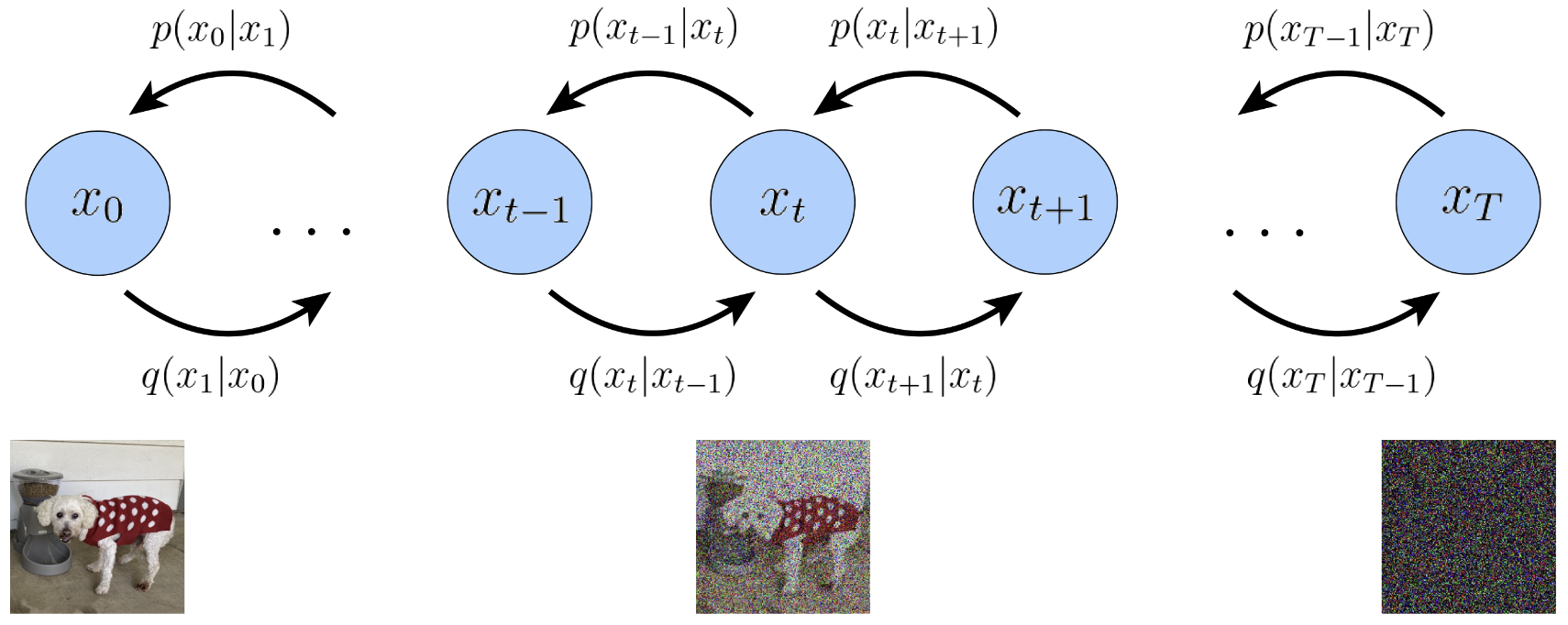
What distinguishes diffusion models from other types of latent variable models is that the approximate posterior $q(x_{1:T}|x_0)$, called the forward process or diffusion process, is fixed to a Markov chain that gradually adds Gaussian noise to the data according to a variance schedule.

Diffusion Process

For a diffusion process from $x_{t-1}$ to $x_t$,

$$x_t={\alpha }_t{x}_{t-1}+{\beta }_t{ϵ}_t,{ϵ}_t\sim \mathcal{N}(0,I)$$

where ${\alpha }_t,{\beta }_t>0$ and ${\alpha }_t^2+{\beta }_t^2=1$. Generally, ${\beta }_t$ always close to $0$ and can be considered as noise degree and ${ϵ}_t$ is the Gaussian noise to diffuse $x_{t-1}$.

Thus we can get:

$$\begin{array}{rl}{x}_t& ={\alpha }_t{x}_{t-1}+{\beta }_t{ϵ}_t\\ & \\ & ={\alpha }_t({\alpha }_{t-1}{x}_{t-2}+{\beta }_{t-1}{ϵ}_{t-1})+{\beta }_t{ϵ}_t\\ & \\ & =\dots \\ & \\ & =({\alpha }_t\cdots {\alpha }_1)x_0+({\alpha }_t\cdots {\alpha }_2){\beta }_1{ϵ}_1+({\alpha }_t\cdots {\alpha }_3){\beta }_2{ϵ}_2+\cdots +{\alpha }_t{\beta }_{t-1}{ϵ}_{t-1}+{\beta }_t{ϵ}_t\end{array}$$

Since ${ϵ}_t\sim \mathcal{N}(0,I)$, so $({\alpha }_t\cdots {\alpha }_2){\beta }_1{ϵ}_1\sim \mathcal{N}(0,({\alpha }_t\cdots {\alpha }_2{)}^2{\beta }_1^2)$, so as others. Thus $({\alpha }_t\cdots {\alpha }_2){\beta }_1{ϵ}_1+({\alpha }_t\cdots {\alpha }_3){\beta }_2{ϵ}_2+\cdots +{\alpha }_t{\beta }_{t-1}{ϵ}_{t-1}+{\beta }_t{ϵ}_t\sim \mathcal{N}(0,({\alpha }_t\cdots {\alpha }_2{)}^2{\beta }_1^2+\cdots +{\alpha }_t^2{\beta }_{t-1}^2+{\beta }_t^2)$.

When ${\alpha }_t^2+{\beta }_t^2=1$,

$$({\alpha }_t\cdots {\alpha }_1{)}^2+({\alpha }_t\cdots {\alpha }_2{)}^2{\beta }_1^2+({\alpha }_t\cdots {\alpha }_3{)}^2{\beta }_2^2+\cdots +{\alpha }_t^2{\beta }_{t-1}^2+{\beta }_t^2=1$$

So $x_t={\bar{\alpha }}_t{x}_0+{\bar{\beta }}_t\overline{{ϵ}_t}$, where ${\overline{ϵ}}_t\sim \mathcal{N}(0,I)$, ${\bar{\alpha }}_t=({\alpha }_t\cdots {\alpha }_1),{\bar{\beta }}_t=\sqrt{1-({\alpha }_t\cdots \alpha 1{)}^2}$.

Reverse Process

We are trying to minimize the distance between original image $x_{t-1}$ and de-noised image $\theta (x_t)$, i.e.:

\begin{aligned} \mathcal{L} &= || x_{t-1} - \theta(x_t) ||^2 \\\\ &= || \frac{1}{\alpha_t}(x_t - \beta_t \epsilon_t) - \theta(x_t) ||^2 \\\\ &= || \frac{1}{\alpha_t}(x_t - \beta_t \epsilon_t) - \frac{1}{\alpha}(x_t - \beta_t \epsilon_{\theta}(x_t, t)) ||^2 \\\\ &= \frac{\beta_t^2}{\alpha_t^2} || \epsilon_t - \epsilon_{\theta}(x_t, t) || ^2 \\\\ &\approx || \epsilon_t - \epsilon_{\theta}(\alpha_t x_{t-1} + \beta_t \epsilon_t, t) || ^2 \\\\ &= || \epsilon_t - \epsilon_{\theta}(\alpha_t (\bar_{\alpha}_{t-1} x_0 + \bar{\beta}_{t-1}\bar{\epsilon}_{t-1}) + \beta_t \epsilon_t, t) || ^2 \\\\ &= || \epsilon_t - \epsilon_{\theta}(\bar{\alpha}_t x_0 + \alpha_t \bar{\beta}_{t-1}\bar{\epsilon}_{t-1} + \beta_t\epsilon_t, t) || ^2 \end{aligned}

We resample $x_t$ without ${\overline{ϵ}}_t$ because ${ϵ}_t$ and ${\overline{ϵ}}_t$ are not independent.

Currently we have four variable need to sample: $x_0$, ${ϵ}_t$, ${\overline{ϵ}}_t$ and $t$. We can use a trick to reduce the variance of training by combining ${ϵ}_t$ and ${\overline{ϵ}}_t$: