Reinforcement Learning
Key Concepts
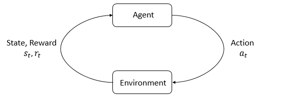
States and Observations
- A state $s$ is a complete description of the state of the world. There is no information about the world which is hidden from the state. An observation $o$ is a partial description of a state, which may omit information.
- When the agent is able to observe the complete state of the environment, we say that the environment is fully observed. When the agent can only see a partial observation, we say that the environment is partially observed.
Actions
- Some environment, like Atari and Go, have discrete action space. only a finite number of moves are available to the agent.
- Other environments, like where the agent controls a robot in a physical world, have continuous action spaces.
Policies
- A policy is a rule used by an agent to decide what actions to take.
- Deterministic Policies output deterministic/specific action values.
-
Stochastic Policies output distribution where action values can be sampled from.
- # Categorical Policies for discrete action space.
- # Stochastic Policies for continuous action space.
Trajectories
A trajectory τ is a sequence of states and actions in the world,
\[ \tau = (s_0, a_0, s_1, a_1, ...), \]
where $s_0 \sim \rho_0(\cdot)$, $a_t = \pi(s_t)$, and $s_{t+1} = P(s_t, a_t)$.
Rewards
The reward function $R$ is critically important in reinforcement learning. It depends on the current state of the world, the action just taken, and the next state of the world:
\[ r_t = R(s_t, a_t, s_{t+1}) \]
Return
One kind of return is the finite-horizon undiscounted return, which is just the sum of rewards obtained in a fixed window of steps:
\[ R(\tau) = \sum_{t=0}^T r_t. \]
Objectives
The goal in RL is to select a policy which maximizes expected return when the agent acts according to it.
Let's suppose that both the environment transitions and the policy are stochastic. In this case, the probability of a T-step trajectory is:
\[ P(\tau|\pi) = \rho_0 (s_0) \prod_{t=0}^{T-1} P(s_{t+1} | s_t, a_t) \pi(a_t | s_t). \]
The expected return, denoted by $J(\pi)$, is then:
\[ J(\pi) = \int_{\tau} P(\tau|\pi) R(\tau) = \mathbb{E}{\tau\sim \pi}{R(\tau)}. \]
The central optimization problem in RL can then be expressed by
\[ \pi^* = \arg \max_{\pi} J(\pi), \]
with $\pi^*$ being the optimal policy.
On-Policy Value Function
The On-Policy Value Function, $V^{\pi}(s)$, which gives the expected return if you start in state s and always act according to policy $\pi$:
\[ V^{\pi}(s) = \mathbb{E}_{\tau \sim \pi}[{R(\tau)\left| s_0 = s\right.}] \]
On-Policy Action-Value Function
The On-Policy Action-Value Function, $Q^{\pi}(s,a)$, which gives the expected return if you start in state $s$, take an arbitrary action $a$ (which may not have come from the policy), and then forever after act according to policy $\pi$:
\[ Q^{\pi}(s,a) = \mathbb{E}_{\tau \sim \pi}[{R(\tau)\left| s_0 = s, a_0 = a\right.}] \]
Bellman Equation
The Bellman equations for the on-policy value functions are
$\begin{aligned} V^{\pi}(s) &= \mathbb{E}_{a \sim \pi, s'\sim P} [r(s,a) + \gamma V^{\pi}(s')], \\ Q^{\pi}(s,a) &= \mathbb{E}_{s'\sim P} [r(s,a) + \gamma \mathbb{E}{a'\sim \pi}{Q^{\pi}(s',a')}], \end{aligned}$
where $s' \sim P$ is shorthand for $s' \sim P(\cdot |s,a)$, indicating that the next state $s'$ is sampled from the environment’s transition rules; $a \sim \pi$ is shorthand for $a \sim \pi(\cdot|s)$; and $a' \sim \pi$ is shorthand for $a' \sim \pi(\cdot|s')$.
The Bellman equations for the optimal value functions are
$\begin{aligned} V^*(s) &= \max_a \mathbb{E}_{s'\sim P}[{r(s,a) + \gamma V^*(s')}], \\ Q^*(s,a) &= \mathbb{E}_{s'\sim P}[{r(s,a) + \gamma \max_{a'} Q^*(s',a')}]. \end{aligned}$
Advantage
The advantage function $A^{\pi}(s,a)$ corresponding to a policy $\pi$ describes how much better it is to take a specific action $a$ in state $s$, over randomly selecting an action according to $\pi(\cdot|s)$, assuming you act according to $\pi$ forever after. Mathematically, the advantage function is defined by
\[ A^{\pi}(s,a) = Q^{\pi}(s,a) - V^{\pi}(s). \]
Kinds of RL Algorithms

One of the most important branching points in an RL algorithm is the question of whether the agent has access to (or learns) a model of the environment. By a model of the environment, we mean a function which predicts state transitions and rewards. Algorithms which use a model are called # Model Based RL, and those that don’t are called # Model Free RL.