Denoising Diffusion Probabilistic Models
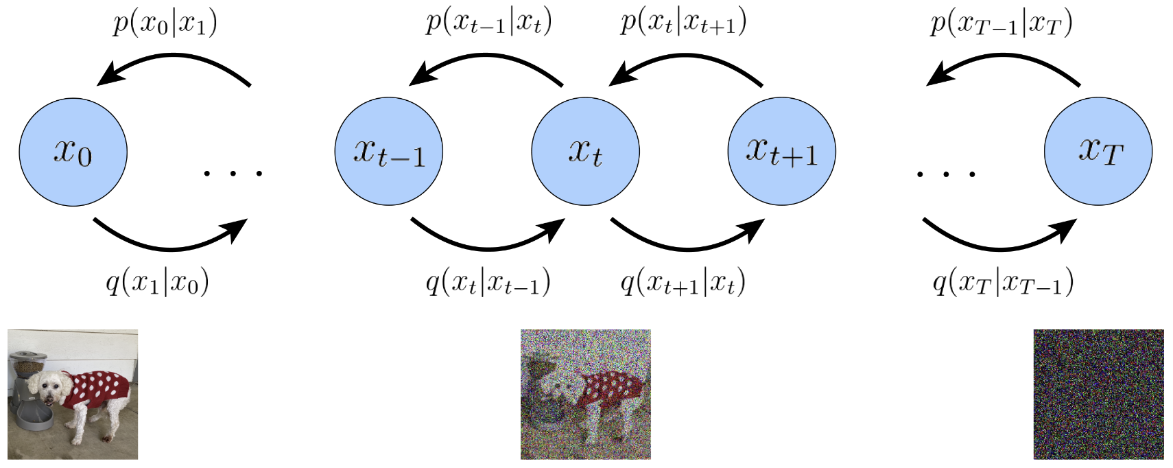
Diffusion models are latent variable models of the form $p_{\theta} := \int p_{\theta}(x_{0:T}) dx_{1:T}$, where $x_1, \cdots, x_T$ are latents of the same dimensionality as the data $x_0 \sim q(x_0)$. $x_0$ represents true data observations such as natural images, $x_T$ represents pure Gaussian noise, and $x_t$ is an intermediate noisy version of $x_0$. The joint distribution $p_{\theta}(x_{0:T})$ is called the reverse process, and it is defined as a Markov chain (shown in Fig.1) with learned Gaussian transitions starting at $p(x_T) = \mathcal{N}(x_T; 0, I)$:
\[ p_{\theta}(x_{0:T}) := p(x_T) \prod_{t=1}^T p_{\theta}(x_{t-1} | x_t) \]
where $p_{\theta}(x_{t-1}|x_t) := \mathcal{N}(x_{t-1}; \mu_{\theta}(x_t, t), \Sigma_{\theta}(x_t, t))$.
What distinguishes diffusion models from other types of latent variable models is that the approximate posterior $q(x_{1:T}|x_0)$, called the forward process or diffusion process, is fixed to a Markov chain that gradually adds Gaussian noise to the data according to a variance schedule.
Diffusion Process
For a diffusion process from $x_{t-1}$ to $x_t$,
\[ x_t = \alpha_t x_{t-1} + \beta_t \epsilon_t, \epsilon_t \sim \mathcal{N}(0, I) \]
where $\alpha_t, \beta_t > 0$ and $\alpha_t^2 + \beta_t^2 = 1$. Generally, $\beta_t$ always close to $0$ and can be considered as noise degree and $\epsilon_t$ is the Gaussian noise to diffuse $x_{t-1}$.
Thus we can get:
$\begin{aligned} x_t &= \alpha_t x_{t-1} + \beta_t \epsilon_t \\ &= \alpha_t (\alpha_{t-1}x_{t-2} + \beta_{t-1}\epsilon_{t-1}) + \beta_t\epsilon_t \\ &= \dots \\ &= (\alpha_t \cdots \alpha_1)x_0 + (\alpha_t \cdots \alpha_2)\beta_1\epsilon_1 + (\alpha_t \cdots \alpha_3) \beta_2 \epsilon_2 + \cdots + \alpha_t\beta_{t-1}\epsilon_{t-1} + \beta_t\epsilon_t \end{aligned}$
Since $\epsilon_t \sim \mathcal{N}(0, I)$, so $(\alpha_t \cdots \alpha_2)\beta_1\epsilon_1 \sim \mathcal{N}(0, (\alpha_t \cdots \alpha_2)^2\beta_1^2)$, so as others. Thus $(\alpha_t \cdots \alpha_2)\beta_1\epsilon_1 + (\alpha_t \cdots \alpha_3) \beta_2 \epsilon_2 + \cdots + \alpha_t\beta_{t-1}\epsilon_{t-1} + \beta_t\epsilon_t \sim \mathcal{N}(0, (\alpha_t \cdots \alpha_2)^2\beta_1^2 + \cdots + \alpha_t^2\beta_{t-1}^2 + \beta_t^2)$.
When $\alpha_t^2 + \beta_t^2 = 1$,
\[ (\alpha_t \cdots \alpha_1)^2 + (\alpha_t \cdots \alpha_2)^2\beta_1^2 + (\alpha_t \cdots \alpha_3)^2\beta_2^2 + \cdots + \alpha_t^2\beta_{t-1}^2 + \beta_t^2 = 1 \]
So $x_t = \bar{\alpha}_t x_0 + \bar{\beta}_t \bar{\epsilon_t}$, where $\bar{\epsilon}_t \sim \mathcal{N}(0, I)$, $\bar{\alpha}_t = (\alpha_t \cdots \alpha_1), \bar{\beta}_t = \sqrt{1 - (\alpha_t \cdots \alpha1)^2}$.
Reverse Process
We are trying to minimize the distance between original image $x_{t-1}$ and de-noised image $\theta(x_t)$, i.e.:
$\begin{aligned}
\mathcal{L}
&= \bigl\|xt-1 - θ(x_t)\bigr\|_2^2
&= \Bigl\|\tfrac{1}{α_t}\bigl(x_t - β_t ε_t\bigr) - θ(x_t)\Bigr\|_2^2
\qquad\text{(since }x_t=α_t xt-1+β_tε_t\text{)}
&= \Bigl\|\tfrac{1}{α_t}\bigl(x_t - β_t ε_t\bigr)
- \tfrac{1}{α_t}\bigl(x_t - β_t \,εθ(x_t,t)\bigr)\Bigr\|_2^2 \\
&= \tfrac{β_t^2}{α_t^2}\,\bigl\|ε_t - εθ(x_t,t)\bigr\|_2^2
&∝ \bigl\|ε_t - εθ(x_t,t)\bigr\|_2^2
\qquad\text{(drop the $t$-dependent factor; constant w.r.t.\ }θ\text{)}
&= \bigl\|ε_t - εθ(α_t xt-1+β_t ε_t,\,t)\bigr\|_2^2
&= \bigl\|ε_t - εθ(\bar{α}_t x_0 + \bar{β}_t \bar{ε}_t,\,t)\bigr\|_2^2,
\end{aligned}$
We resample $x_t$ without $\bar{\epsilon}_t$ because $\epsilon_t$ and $\bar{\epsilon}_t$ are not independent.
Currently we have four variable need to sample: $x_0$, $\epsilon_t$, $\bar{\epsilon}_t$ and $t$. We can use a trick to reduce the variance of training by combining $\epsilon_t$ and $\bar{\epsilon}_t$: