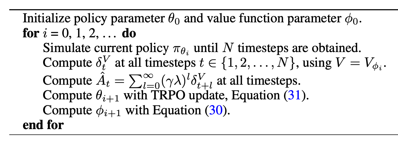
Generalized Advantage Estimate

Policy gradient methods maximize the expected total reward by repeatedly estimating the gradient $g:=\nabla_{\theta} \mathbf{E}[\sum_{t=0}^{\infty}r_{t}]$ . There are several different related expressions for the policy gradient, which have the form

$ g = \mathbf{E}\left[ \sum_{t=0}^{\infty}\Psi_{t}\nabla_{\theta}\log\pi_{\theta}(a_{t}|s_{t}) \right] $

where $\Psi_{t}$ may be one of the follows(All unbiased):

1. $\sum_{t=0}^{\infty}r_{t}$: total reward of the trajectory.
2. $\sum_{t^{\prime}=t}^{\infty}r_{t^{\prime}}$: rewards following action $a_t$.
3. $\sum_{t^{\prime}=t}^{\infty}r_{t^{\prime}}-b(s_{t})$: baselined version of previous formula.
4. $Q^{\pi}(s_{t},a_{t})$ state-action value function.
5. $A^{\pi}(s_{t}, a_{t})$ advantage function.
6. $r_t + V^{\pi}(s_{t+1}) - V^{\pi}(s_{t})$: TD residual.

The first three formulas are deduced in # Policy Gradient.

The latter formulas use the definitions: $ V^{\pi}(s_t) := \mathbf{E}_{s_{t+1}:\infty,a_{t}:\infty} \left[ \sum_{l=0}^{\infty}r_{t+l} \right] $

$ Q^{\pi}(s_t,a_t) := \mathbf{E}_{s_{t+1}:\infty,a_{t+1}:\infty} \left[ \sum_{l=0}^{\infty}r_{t+l} \right] $

$ A^{\pi}(s_t, a_t) := Q^{\pi}(s_t, a_t) - V^{\pi}(s_t) $

The advantage function measures whether or not the action is better or worse than the policy's default behavior. And it's gradient item points in the direction of increased policy if and only if the advantage function $>$ 0.

Then we introduce a parameter $\gamma$ that allow us to reduce variance by downweighting rewards corresponding to delayed effects, at the cost of introducing bias. The discounted value functions are given by:

$ V^{\pi,\gamma}(s_t) := \mathbf{E}_{s_{t+1}:\infty,a_{t}:\infty} \left[ \sum_{l=0}^{\infty}\gamma^{l}r_{t+l} \right] $

$ Q^{\pi,\gamma}(s_t) := \mathbf{E}_{s_{t+1}:\infty,a_{t+1}:\infty} \left[ \sum_{l=0}^{\infty}\gamma^{l}r_{t+l} \right] $

$ A^{\pi\gamma}(s_t, a_t) := Q^{\pi,\gamma}(s_t, a_t) - V^{\pi,\gamma}(s_t) $

It's a biased(but not too biased) estimate of $A^{\pi}$.

And the discounted approximation to the policy gradient is $ g^{\gamma} := \mathbf{E}_{s_{0:\infty},a_{0:\infty}} \left[ \sum_{t=0}^{\infty} A^{\pi,\gamma}(s_t,a_t)\nabla_{\theta}\log\pi_{\theta}(a_t|s_t) \right] $

Here we want to concern about unbiased estimate of $A^{\pi,\gamma}$.

Definition The estimator $\hat{A_{t}}$ is $\gamma$-just if $$ \mathbf{E}_{s_{0:\infty},a_{0:\infty}} \left[ \hat{A_t}(s_{0:\infty})\nabla_{\theta}\log\pi_{\theta}(a_t|s_t) \right] = \mathbf{E}_{s_{0:\infty},a_{0:\infty}} \left[ A^{\pi,\gamma}(s_t,a_t)\nabla_{\theta}\log\pi_{\theta}(a_t|s_t) \right] $$

It follows immediately that if $\hat{A_t}$ is $\gamma$-just, then

$ \mathbf{E}_{s_{0:\infty},a_{0:\infty}} \left[ \sum_{t=0}^{\infty}\hat{A_t}(s_{0:\infty})\nabla_{\theta}\log\pi_{\theta}(a_t|s_t) \right] = g^{\gamma} $

Suppose that $\hat{A_t}$ can be written in the form $\hat{A_t}(s_{0:\infty},a_{0:\infty})=Q_{t}(s_{t:\infty},a_{t:\infty})-b_{t}(s_{0:t},a_{0:t-1})$ such that for all $(s_t,a_t)$, $\mathbf{E}_{s_{t+1:\infty},a_{t+1:\infty}|s_t,a_t}Q_{t}(s_{t:\infty},a_{t:\infty})=Q^{\pi,\gamma}(s_t,a_t)$ then $\hat{A_{t}}$ is $\gamma$-just.

STILL not prove above. Didn't understand the prefix proof in original paper.

It's easy to verify that the following expressions are $\gamma$-just advantage estimators for $\hat{A_t}$:

• $\sum_{l=0}^{\infty}\gamma^{l}r_{t+1}$
• $Q^{\pi,\gamma}(s_t,a_t)$
• $A^{\pi,\gamma}(s_t,a_t)$
• $r_t + \gamma V^{\pi,\gamma}(s_{t+1}) - V^{\pi,\gamma}(s_t)$

Our estimator of policy gradient is $$ \hat{g} = \frac{1}{N}\sum_{n=1}^{N}\sum_{t=0}^{\infty} \hat{A_t^{n}}\nabla_{\theta}\log\pi_{\theta}(a_t^n|s^t_n) $$

where $n$ indexes over a batch of episodes.

Let $V$ be an approximate value function. Define $\delta_t^V=r_t+\gamma V(s_{t+1}) - V(s_t)$, i.e., the TD residual of V with dicounted $\gamma$.

If we have correct value function $V = V^{\pi,\gamma}$, then

\begin{aligned} \mathbf{E}_{s_{t+1}}\left[\sigma_{t}^{V^{\pi,\gamma}}\right] &= \mathbf{E}_{s_{t+1}}\left[ r_t+\gamma V^{\pi,\gamma}(s_{t+1}) - V^{\pi,\gamma}(s_t) \right] \\ &= \mathbf{E}_{s_{t+1}}\left[ Q^{\pi,\gamma}(s_{t}, a_{t}) - V^{\pi,\gamma}(s_t) \right] \\ &= A^{\pi,\gamma}(s_t,a_t) \end{aligned}

However, this estimator is only $\gamma$-just for $V=V^{\pi,\gamma}$, otherwise it will yield biased policy gradient estimates.

Next let us consider taking the sum of $k$ of these $\sigma$ items, which we will denote by $\hat{A_t}^{k}$ $$ \hat{A}_{t}^{(k)}:=\sum_{l=0}^{k-1} \gamma^{l} \delta_{t+l}^{V}=-V\left(s_{t}\right)+r_{t}+\gamma r_{t+1}+\cdots+\gamma^{k-1} r_{t+k-1}+\gamma^{k} V\left(s_{t+k}\right) $$

which is simply the empirical returns minus the value function baseline.

The GAE(generalized advantage estimator) is defined as the exponentially-weighted average of these $k$ -step estimators:

\begin{aligned} \hat{A}_{t}^{\mathrm{GAE}(\gamma, \lambda)} &:=(1-\lambda)\left(\hat{A}_{t}^{(1)}+\lambda \hat{A}_{t}^{(2)}+\lambda^{2} \hat{A}_{t}^{(3)}+\ldots\right) \\ &=(1-\lambda)\left(\delta_{t}^{V}+\lambda\left(\delta_{t}^{V}+\gamma \delta_{t+1}^{V}\right)+\lambda^{2}\left(\delta_{t}^{V}+\gamma \delta_{t+1}^{V}+\gamma^{2} \delta_{t+2}^{V}\right)+\ldots\right) \\ &=(1-\lambda)\left(\delta_{t}^{V}\left(1+\lambda+\lambda^{2}+\ldots\right)+\gamma \delta_{t+1}^{V}\left(\lambda+\lambda^{2}+\lambda^{3}+\ldots\right)\right.\\ &\left.\quad+\gamma^{2} \delta_{t+2}^{V}\left(\lambda^{2}+\lambda^{3}+\lambda^{4}+\ldots\right)+\ldots\right) \\ =&(1-\lambda)\left(\delta_{t}^{V}\left(\frac{1}{1-\lambda}\right)+\gamma \delta_{t+1}^{V}\left(\frac{\lambda}{1-\lambda}\right)+\gamma^{2} \delta_{t+2}^{V}\left(\frac{\lambda^{2}}{1-\lambda}\right)+\ldots\right) \\ =& \sum_{l=0}^{\infty}(\gamma \lambda)^{l} \delta_{t+l}^{V} \end{aligned}

There are two notable special cases of this formula, obtained by setting $\lambda=0$ and $\lambda=1$.

\begin{array}{ll} \operatorname{GAE}(γ, 0): & \hat{A}_t:=δ_t \quad=r_t+γ V≤ft(s_t+1\right)-V≤ft(s_t\right)
\operatorname{GAE}(γ, 1): & \hat{A}_t:=∑_l=0^∞ γ^l δ_t+l=∑_l=0^∞ γ^l r_t+l-V≤ft(s_t\right)

\end{array}

$GAE(\gamma,0)$ is $\gamma$ -just for $V=V^{\pi,\gamma}$ and otherwise induces bias, but it typically has much lower variance. $GAE(\gamma,1)$ is $\gamma$ -just regardless of the accuracy of $V$, but it has high variance due to the sum of terms. Empirically, we find that the best value of $\lambda$ is much lower than the best value of $\gamma$, likely because $\lambda$ introduces far less bias than $\gamma$ for a reasonably accurate value function.

\begin{equation} g^{\gamma} \approx \mathbb{E}\left[\sum_{t=0}^{\infty} \nabla_{\theta} \log \pi_{\theta}\left(a_{t} \mid s_{t}\right) \hat{A}_{t}^{\mathrm{GAE}(\gamma, \lambda)}\right]=\mathbb{E}\left[\sum_{t=0}^{\infty} \nabla_{\theta} \log \pi_{\theta}\left(a_{t} \mid s_{t}\right) \sum_{l=0}^{\infty}(\gamma \lambda)^{l} \delta_{t+l}^{V}\right] \end{equation}

where equality hold s when $\lambda=1$.